The book Concrete Functional Analysis by Richard M. Dudley and Rimas Norvaiša presents some aspects of nonlinear analysis and their applications to probability.
I wanted to get an understanding of the book as it could have been taught to a high school student. Here, I found the following observations by examining via the lens of AI tools.
The idea behind the book is that there is a new measure or yardstick for variation referred to as wiggliness and defined as p-variation. It adds up the size of each little wiggle and raises it to the power of p. Bigger p pays little attention to tiny jitter and more to big moves. This gives a new family of wiggliness meters not just one.
The book demonstrates that with the right p, we can make sense of integrals and calculus style operations even for quite jumpy signals. This lead to a result called the Love-Young inequality, which tells you when an integral  exists and how big it can be based on the p-variation of
  and the q-variation of
  with
with  .
.
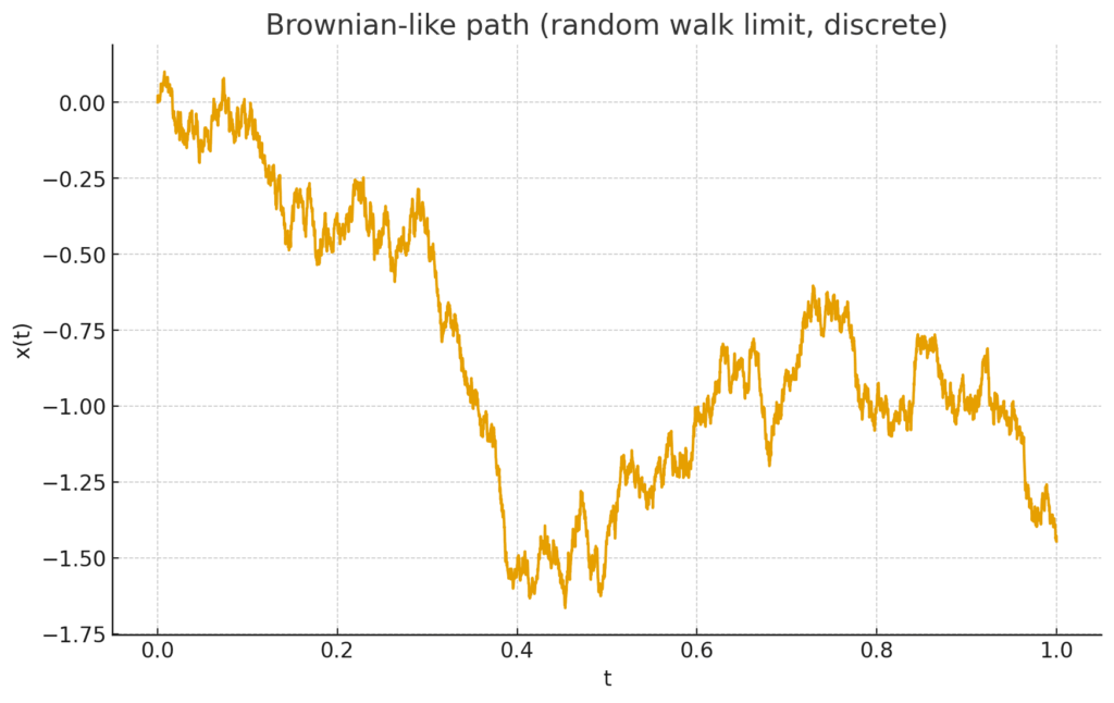
For Brownian motion, a Brownian path has finite p-variation only when  , too wiggly for
  .
.
If one function is “not too wiggly” in the p-variation sense and the other is “not too wiggly” in q-variation with
the integral
exists and is controlled (Love–Young). This is like a cousin of Cauchy–Schwarz/Hölder, but tuned to rough signals. In stats terms: it tells you when you can safely integrate (or “accumulate”) a noisy curve against another without things blowing up.
The book also studies when composition of functions behave smoothly – like a data pipeline where you first transform your variable with  , then apply
  .
.
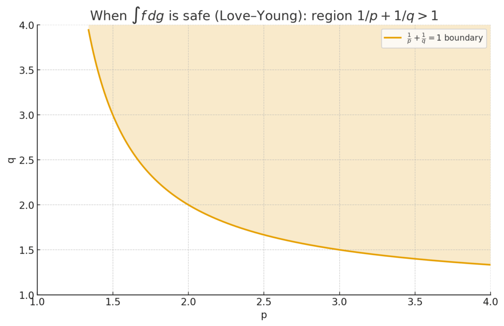
The Love–Young “safe integration” region where .Example: Brownian needs ; pair it with something with, say,  so the inequality holds.
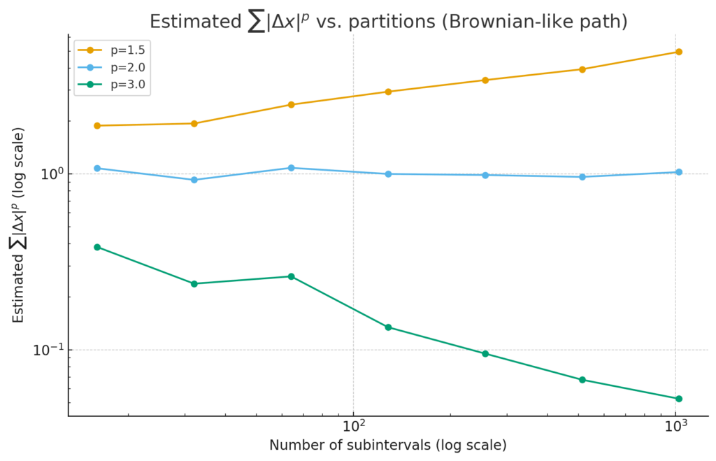
how the estimate  changes as we cut the interval into more and more pieces.
Brownian-like path
p=3 shrinks → for  , the roughness is “tamed,” and p-variation is finite.
p=1.5 grows with refinement → too rough: p-variation “blows up” for  .
.
p=2 hovers around a constant (the borderline).