LEARNING FROM DATA

Why rare variants, and not common variants, are best for therapeutic hypotheses

Although cumulatively common variants appear to explain a large fraction of the heritability of most human traits, they offer little benefit to drug developers. For one, it is quite difficult to pinpoint the culprit genes, much less the culprit variants, and for two the functional consequences are poorly understood.

Relationship between polygenic risk score (x-axis) and standing height (y-axis) in UK Biobank.

Unlike common variants, rare variants offer an alternative view that makes it easier to distinguish causal relationships due to breaking of the correlation structure between variants and the complex trait association support by multiple independent variants.

We’ve written some papers on looking at multiple properties of rare variants to jointly dissect their contribution:
1. by looking at the effect of the genetic variants by protein structure impact prediction;
2. by looking at whether the genetic variants lead to loss of gene function; and
3. by looking at whether information about what is happening to their neighbors is informative about what is happening to you and your relationship to the human trait of interest.

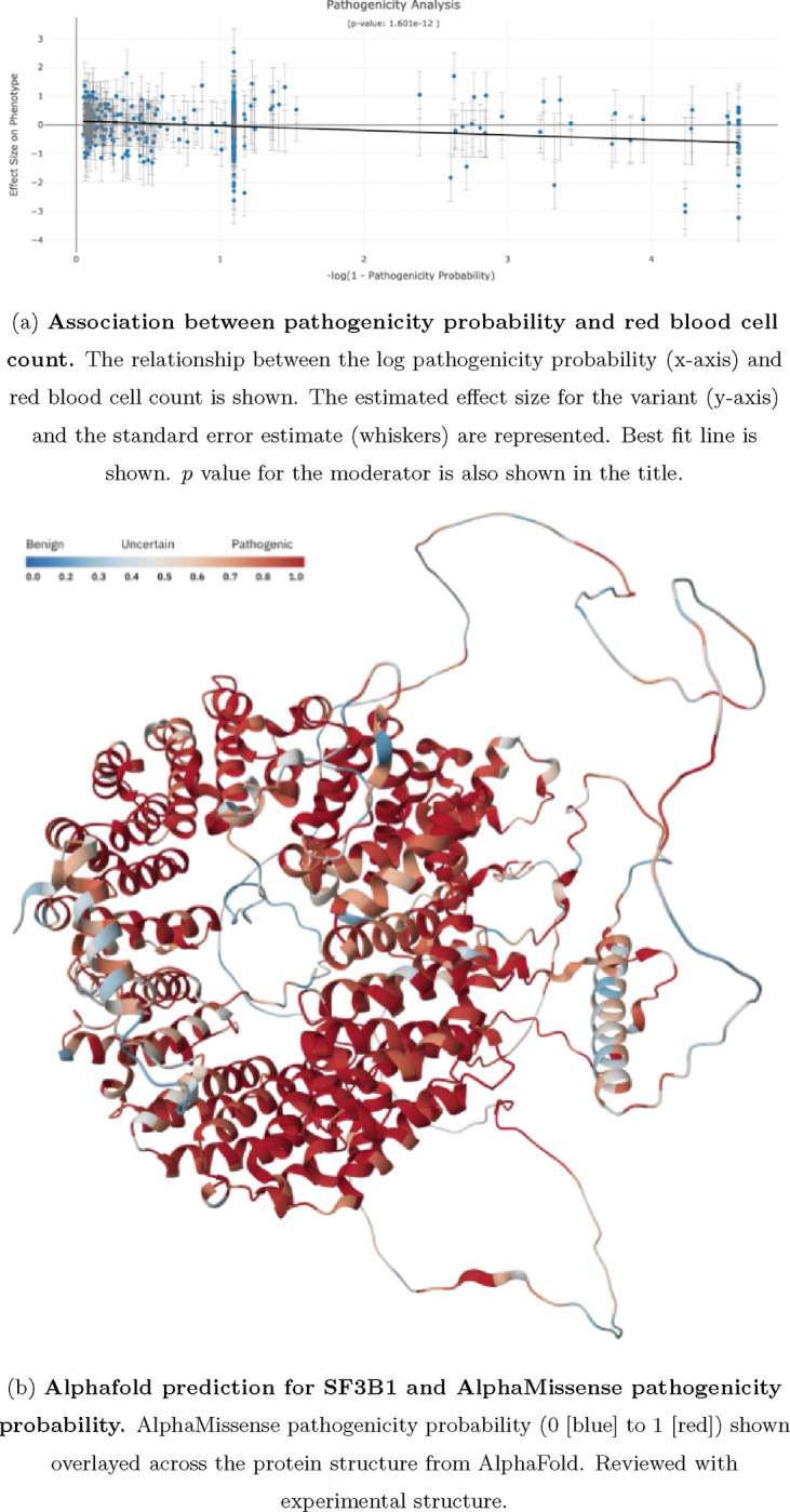
Below is an example where we see that the probability of pathogenicity, i.e. a probability determined by the predicted impact of the mutation on protein folding by a deep learning algorithm, is related to the observed values of red blood cell count in individuals that carry those mutations. The location of mutations that are pathogenic are shown in Figure panel (b).

October 10, 2025
Demographic modeling of population growth

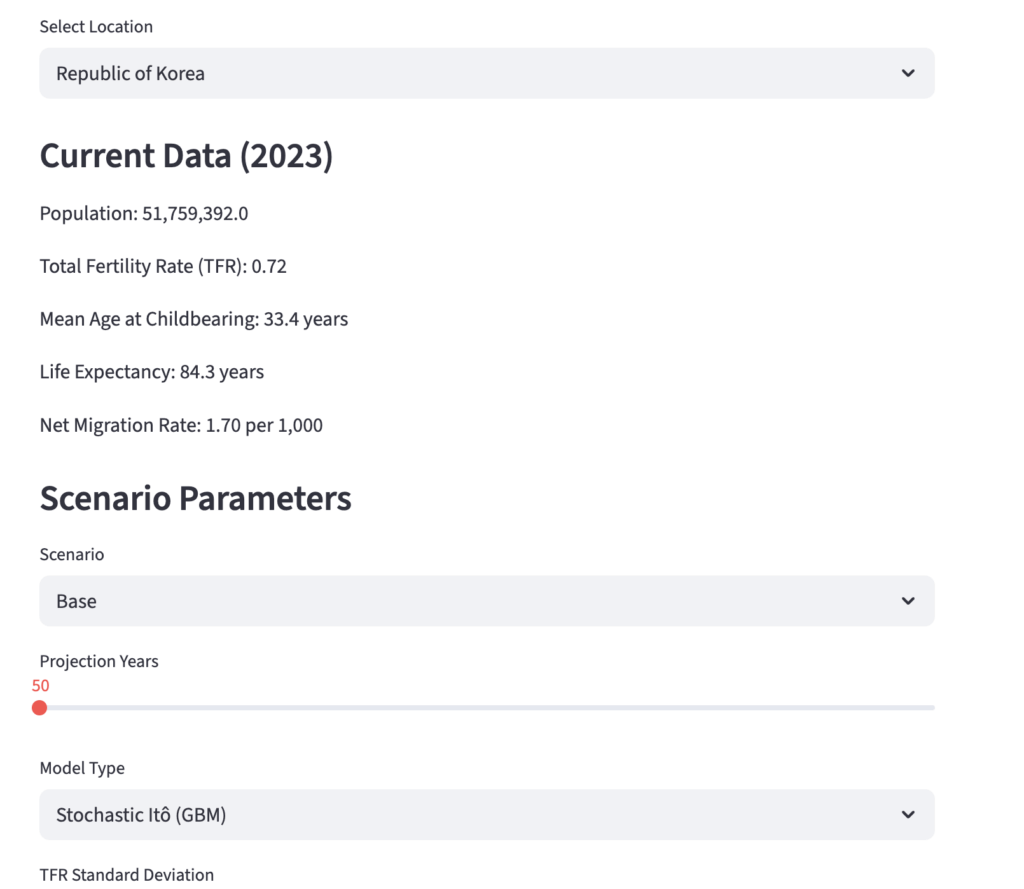
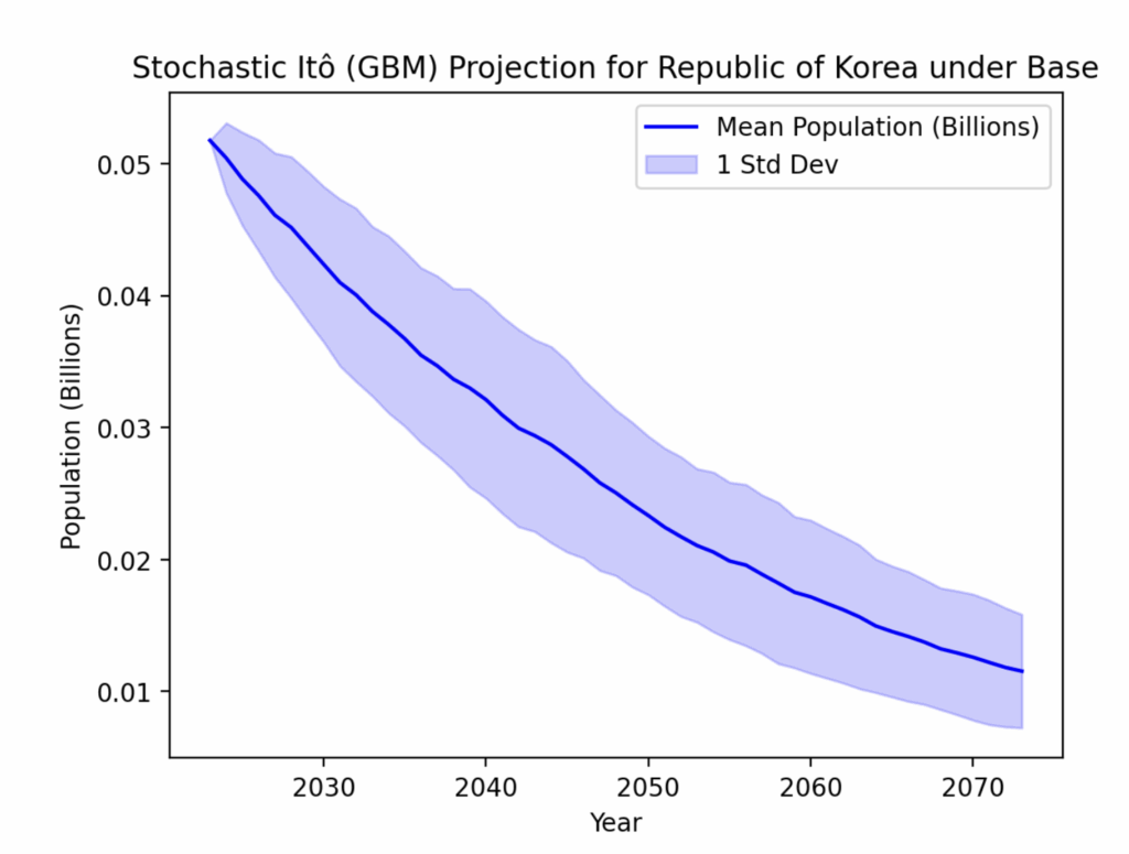
Kiyosi Itô pioneered the theory of stochastic integration and stochastic differential equations. I used AI and the United Nations growth data to project population growth across various countries given migration patterns, fertility rates, etc.

https://demographic.streamlit.app/

Here is a technical report on the demographic modeling work.

October 7, 2025
Brownian motion and martingales and their relations
Brownian motion

Brownian motion is defined as a stochastic process $\{X_t\}_{t \geq 0}$ which is Gaussian, i.e. such that for any $0 \leq t_0 < t_1 < \cdots < t_n$ , $X_{t_j}$ for $j = 0, 1, \cdots, n$ have a jointly Gaussian (normal distribution), $\mathbb{E}X_t = 0$ for all $t$ , and the covariance is $\mathbb{E}X_sX_t = \min(s,t)$ for all $s, t \geq 0$ . A normal distribution is uniquely determined by its mean vector $\mu$ and covariance matrix $C$ . Each $X_t$ has a normal distribution $\mathcal{N}(0, t)$ .

Brownian motion – multiple sample paths from t = 0 to t = 5.

Density at t = 2.5.

It follows from the definition that Brownian motion has independent increments, in other words whenever $0 \leq s < t \leq u < v$ , $X_t - X_s$ and $X_v - X_u$ are independent.

A consequence of the definition is that for any $c > 0$ , the process $X_{c^2t}/ c$ is also a Brownian motion.

By a therorem of Norbert Wiener, Brownian motion can be chosen such that with probability 1 (or for all $w$ ), $X_t(w)$ is continuous as a function of $t$ . a Brownian motion with this property is called the standard Brownian motion.

A Markov time $\tau$ for Brownian motion is defined as a random variable $\tau \geq 0$ such that for each $t > 0$ , the event $\{ \tau < t\}$ is a function of $X_s$ for $0 \leq s \eq t$ .

The strong Markov property of Brownian motion says that if $\tau$ is a Markov time such that $\math{P}(\tau < \infty) > 0$ , then conditional on $\tau < \infty$ , the process $V_{t} \def X_{\tau + t} - X_{\tau}$ for $t \geq 0$ is itself a Brownian motion and is independent of $X_s$ for $s \leq \tau$ .

Using the strong Markov property one can prove the reflection principle for Brownian motion: for any $b > 0$ and $t > 0$ , the probability that $X_s \geq b$ for some $s$ with $0 < s \leq t$ equals $2\mathbb{P}\left(X_t \geq b\right)$ .

What may be called “Wald’s identity“ for Brownian motion says that if $\tau$ is a Markov time with $\mathbb{E}\left[\tau\right] < \infty$ , and so $\tau < \infty$ with probability 1, $\mathbb{E}\left[X_{\tau}\right] = 0$ and $\mathbb{E}\left[X_{\tau}^2\right] = \mathbb{E}\left[\tau\right]$ .

The Brownian Bridge is a Gaussian process $Y_t$ defined for $0 \leq t \leq 1$ with $\mathbb{E}\left[Y_t\right] \equiv 0$ and covariance $\mathbb{E}\left[Y_SY_t\right] = s\left(1 - t\right)$ for $0 \leq s \leq t \leq 1$ .

The path starts and ends at 0 (a.s.).
The dashed curves plot the $\pm 2\sqrt{t(1-t)}$ band (two standard deviations), and the dotted line marks the zero mean.
Note that $Y_0=Y_1=0$ a.s., and the fluctuations are largest near $t=\tfrac12$ .

Relations between the Brownian motion and Brownian bridge:
- If $\{X_t\}_{t \geq 0}$ is a Brownian motion then $Y_t = X_t - tX_1$ for $0 \leq t \leq 1$ is a Brownian bridge, which is independent of $X_1$ . This shows that $Y_t$ also can (and will) be taken to be continuity as a function of $t$ .
- Conversely, if $\{Y_t\}_{0 \leq t \leq 1}$ is a Brownian bridge and $Z$ is a $\mathcal{N}\left(0, 1\right)$ variable independent of $\{Y_t\}_{0 \leq t \leq 1}$ then $Y_t + t Z$ has the distribution of Brownian motion for $0 \leq t \leq 1$ .
- The conditional distribution of $\{X_t\}_{0 \leq t \leq 1}$ given that $|X_1| < \epsilon$ converges to that of $\{Y_t\}_{0 \leq t \leq 1$ as $\epsilon \downarrow 0$ .
- If $\{Y_t\}_{0\leqt\leq1}$ is a Brownian bridge and $X_t := (1 + t) Y_{t/ (1 + t)}$ then $\{ X_t \}_{t \geq 0}$ is a Brownian motion.
Brownian motion (BM) — where it shows up
- Physics & PDEs: Diffusion of particles; probabilistic solution of the heat equation; harmonic measure & potential theory.
- Finance: Geometric BM for asset prices; correlated BMs in stochastic volatility (e.g., Heston); first-passage ideas for default/credit models; Monte Carlo pricing.
- Statistics & sequential analysis: Likelihood-ratio tests/SPRT; drift-diffusion models for decision making; estimation of diffusion parameters; functional CLT (random walk ⇒ BM).
- Machine learning & MCMC: Langevin Monte Carlo; score-based/diffusion generative models (continuous-time SDE viewpoint).
- Biology & neuroscience: Wright–Fisher diffusion (genetic drift); membrane-potential and evidence-accumulation models (first-passage times).
- Queues, control, and signals: Heavy-traffic limits (Reflected BM); Kalman–Bucy filtering (continuous time); integrated white noise as a model for 1/f21/f^21/f2-like signals.
Brownian bridge (BB) — why it’s special

A BB is BM on [0,1]conditioned to be 0 at t=1: Yt=Bt−tB1
- Goodness-of-fit tests: The exact null distributions of Kolmogorov–Smirnov, Cramér–von Mises, and Anderson–Darling statistics are functionals of a BB.
- Empirical process theory: Donsker’s theorem ⇒ centered empirical CDF processes converge to a BB; yields asymptotic CIs/bands for distribution functions and QQ-plots.
- Conditioned path sampling: “Diffusion bridges” in Bayesian inference, particle filters, and SDE calibration when you know endpoints (e.g., smoothing between observations).
- Finance (variance reduction): Brownian-bridge corrections in Monte Carlo for barrier options: between time steps, condition on endpoints to estimate barrier crossings and cut bias/variance.
- Boundary crossing & change-point: Many suprema/infima of centered cumulative sums have BB limits, giving p-values and thresholds for change-point and scan statistics.
- Random geometry/combinatorics: BB/bridges underpin Brownian excursions, which connect to random trees (Aldous’ CRT) and scaling limits in random maps.
Let $\{Y_t\}_{0 \leq t \leq1}$ be a Brownian bridge and $b > 0$ . Then,

(a) the probability that $Y_t \geq b$ for some $t$ , which is the same that probability that $Y_t = b$ for some $t$ by sample continuity and the intermediate value theorem, equals $\exp(-2b^2)$ .

(b) the probability that $|Y_t| \geq b$ for some $t$ , which is the same as the probability that $|Y_t| = b$ for some $t$ , equals $2\sum_{j = 1}^{\infty} (-1)^{j - 1}exp(-2j^2b^2)$ . The series converges quite fast except for small b.

For a Brownian motion $\{X_t\}_{t \geq 0}$ and two real numbers $a$ and $b$ , let $\tau$ be the least time $t$ such that $X_t = at + b$ , if such a $t$ exists, or $+\infty$ otherwise. Then $\tau$ is a Markov time.

(a) If $b = 0$ then $\tau \equiv 0$ .

(b) If $a = 0 \neq b$ then $\mathbb{P}(\tau < \infty ) = 1$ but $\mathbb{E}\left[\tau\right] = +\infty$ , otherwise we’d get a contradiction to the Wald identity $\mathbb{E}\left[X_{\tau}\right] = 0$ .

(c) If $ab < 0$ then $\mathbb{P}(\tau < \infty ) = 1$ and $\mathbb{E}\left[X_{\tau}\right] = -\frac{a}{b}$ .

(d) If $ab > 0$ then $0 < \mathbb{P}(\tau < \infty) = e^{-2ab} < 1$ .

Martingales

Let $\{X_n\}_{n \geq 1}$ be a sequence of random variables. Let $\mathcal{F}_n$ be a collection of random variables such that $\mathcal{F}_m \subset \mathcal{F}_n$ for $m \leq n$ and $X_n \in \mathcal{F}_n$ for each $n$ . Then, $\{X_n\}$ is called a martingale sequence if whenever $m < n$ , $X_m = \mathbb{E}(X_n | \mathcal{F}_m)$ , or a submartingale sequence if $X_m \leq \mathbb{E}(X_n | \mathcal{F}_m)$ , or a supermartingale sequence if $X_m \geq \mathbb{E}(X_n | \mathcal{F}_m)$ .

To make the collection $\mathcal{F}_n$ as small as possible one can and often will take $\mathcal{F}_n = \{X_1, X_2, \dots, X_n\}$ .

A stopping time for a martingale (or sub- or supermartingale) sequence is a positive integer-valued random variable $\tau$ such that for each $n = 1, 2, \dots,$ the event $\{\tau \leq n\}$ is a function of the variables in $\mathcal{F}_{n}$ .

Optional stopping. Let $\{X_n\}_{n \geq 1}$ be a martingale sequence for $\mathcal{F}_{n} = \{X_1, \dots, X_n \}$ . Let $N < \infty$ and let $\sigma$ and $\tau$ be two stopping times for $\{\mathcal{F}_n\}_{n \geq 1}$ such that $\sigma \leq \tau \leq N$ with probability 1. Then $\mathbb{E}(X_{\tau} | X_j , j \leq \sigma) = X_{\sigma}$ . For a submartingale or supermartingale, the equality is replaced by $\geq$ or $\leq$ respectively.

Doob’s maximal inequality. Let $\{X_j\}_{j \geq 1}$ be a submartingale sequence, let $M > 0$ , and let $A(M, n)$ be the event $\{max_{1 \leq j \leq n} X_j \geq M \}$ . Then

$MP(A(M, n)) \leq \mathbb{E}(X_n \mathds{1}_{A(M, n)}) \leq \mathbb{E}(\max(X_n, 0))$

Let $X_n \geq 0$ for all $n$ and suppose $\{X_n \}$ form a supermartingale with respect to $\mathcal{F}_n = \{X_1, \dots, X_n\}$ . Let $\sigma \leq \tau \leq +\infty$ be stopping times for $\{X_n \}$ . Then

$\mathbb{E}(X_{\tau}\mathds{1}_{\tau < \infty} | j \leq \sigma) \leq X_{\sigma}\mathds{1}_{\sigma < \infty}$
.

Taking expectations of both sides gives

$\mathbb{E}(X_{\tau}\mathds{1}_{\tau < \infty}) \leq \mathbb{E}(X_{\sigma}\mathds{1}_{\sigma < \infty}).$

This is an integration of notes from Stochastic Processes with AI. Pretty impressive.
October 7, 2025