admin – Page 5 – LEARNING FROM DATA

Brownian motion and martingales and their relations

Brownian motion

Brownian motion is defined as a stochastic process $\{X_t\}_{t \geq 0}$ which is Gaussian, i.e. such that for any $0 \leq t_0 < t_1 < \cdots < t_n$ , $X_{t_j}$ for $j = 0, 1, \cdots, n$ have a jointly Gaussian (normal distribution), $\mathbb{E}X_t = 0$ for all $t$ , and the covariance is $\mathbb{E}X_sX_t = \min(s,t)$ for all $s, t \geq 0$ . A normal distribution is uniquely determined by its mean vector $\mu$ and covariance matrix $C$ . Each $X_t$ has a normal distribution $\mathcal{N}(0, t)$ .

It follows from the definition that Brownian motion has independent increments, in other words whenever $0 \leq s < t \leq u < v$ , $X_t - X_s$ and $X_v - X_u$ are independent.

A consequence of the definition is that for any $c > 0$ , the process $X_{c^2t}/ c$ is also a Brownian motion.

By a therorem of Norbert Wiener, Brownian motion can be chosen such that with probability 1 (or for all $w$ ), $X_t(w)$ is continuous as a function of $t$ . a Brownian motion with this property is called the standard Brownian motion.

A Markov time $\tau$ for Brownian motion is defined as a random variable $\tau \geq 0$ such that for each $t > 0$ , the event $\{ \tau < t\}$ is a function of $X_s$ for $0 \leq s \eq t$ .

The strong Markov property of Brownian motion says that if $\tau$ is a Markov time such that $\math{P}(\tau < \infty) > 0$ , then conditional on $\tau < \infty$ , the process $V_{t} \def X_{\tau + t} - X_{\tau}$ for $t \geq 0$ is itself a Brownian motion and is independent of $X_s$ for $s \leq \tau$ .

Using the strong Markov property one can prove the reflection principle for Brownian motion: for any $b > 0$ and $t > 0$ , the probability that $X_s \geq b$ for some $s$ with $0 < s \leq t$ equals $2\mathbb{P}\left(X_t \geq b\right)$ .

What may be called “Wald’s identity“ for Brownian motion says that if $\tau$ is a Markov time with $\mathbb{E}\left[\tau\right] < \infty$ , and so $\tau < \infty$ with probability 1, $\mathbb{E}\left[X_{\tau}\right] = 0$ and $\mathbb{E}\left[X_{\tau}^2\right] = \mathbb{E}\left[\tau\right]$ .

The Brownian Bridge is a Gaussian process $Y_t$ defined for $0 \leq t \leq 1$ with $\mathbb{E}\left[Y_t\right] \equiv 0$ and covariance $\mathbb{E}\left[Y_SY_t\right] = s\left(1 - t\right)$ for $0 \leq s \leq t \leq 1$ .

The path starts and ends at 0 (a.s.).
The dashed curves plot the $\pm 2\sqrt{t(1-t)}$ band (two standard deviations), and the dotted line marks the zero mean.
Note that $Y_0=Y_1=0$ a.s., and the fluctuations are largest near $t=\tfrac12$ .

Relations between the Brownian motion and Brownian bridge:

If $\{X_t\}_{t \geq 0}$ is a Brownian motion then $Y_t = X_t - tX_1$ for $0 \leq t \leq 1$ is a Brownian bridge, which is independent of $X_1$ . This shows that $Y_t$ also can (and will) be taken to be continuity as a function of $t$ .
Conversely, if $\{Y_t\}_{0 \leq t \leq 1}$ is a Brownian bridge and $Z$ is a $\mathcal{N}\left(0, 1\right)$ variable independent of $\{Y_t\}_{0 \leq t \leq 1}$ then $Y_t + t Z$ has the distribution of Brownian motion for $0 \leq t \leq 1$ .
The conditional distribution of $\{X_t\}_{0 \leq t \leq 1}$ given that $|X_1| < \epsilon$ converges to that of $\{Y_t\}_{0 \leq t \leq 1$ as $\epsilon \downarrow 0$ .
If $\{Y_t\}_{0\leqt\leq1}$ is a Brownian bridge and $X_t := (1 + t) Y_{t/ (1 + t)}$ then $\{ X_t \}_{t \geq 0}$ is a Brownian motion.

Brownian motion (BM) — where it shows up

Physics & PDEs: Diffusion of particles; probabilistic solution of the heat equation; harmonic measure & potential theory.
Finance: Geometric BM for asset prices; correlated BMs in stochastic volatility (e.g., Heston); first-passage ideas for default/credit models; Monte Carlo pricing.
Statistics & sequential analysis: Likelihood-ratio tests/SPRT; drift-diffusion models for decision making; estimation of diffusion parameters; functional CLT (random walk ⇒ BM).
Machine learning & MCMC: Langevin Monte Carlo; score-based/diffusion generative models (continuous-time SDE viewpoint).
Biology & neuroscience: Wright–Fisher diffusion (genetic drift); membrane-potential and evidence-accumulation models (first-passage times).
Queues, control, and signals: Heavy-traffic limits (Reflected BM); Kalman–Bucy filtering (continuous time); integrated white noise as a model for 1/f21/f^21/f2-like signals.

Brownian bridge (BB) — why it’s special

A BB is BM on [0,1]conditioned to be 0 at t=1: Yt=Bt−tB1

Goodness-of-fit tests: The exact null distributions of Kolmogorov–Smirnov, Cramér–von Mises, and Anderson–Darling statistics are functionals of a BB.
Empirical process theory: Donsker’s theorem ⇒ centered empirical CDF processes converge to a BB; yields asymptotic CIs/bands for distribution functions and QQ-plots.
Conditioned path sampling: “Diffusion bridges” in Bayesian inference, particle filters, and SDE calibration when you know endpoints (e.g., smoothing between observations).
Finance (variance reduction): Brownian-bridge corrections in Monte Carlo for barrier options: between time steps, condition on endpoints to estimate barrier crossings and cut bias/variance.
Boundary crossing & change-point: Many suprema/infima of centered cumulative sums have BB limits, giving p-values and thresholds for change-point and scan statistics.
Random geometry/combinatorics: BB/bridges underpin Brownian excursions, which connect to random trees (Aldous’ CRT) and scaling limits in random maps.

Let $\{Y_t\}_{0 \leq t \leq1}$ be a Brownian bridge and $b > 0$ . Then,

(a) the probability that $Y_t \geq b$ for some $t$ , which is the same that probability that $Y_t = b$ for some $t$ by sample continuity and the intermediate value theorem, equals $\exp(-2b^2)$ .

(b) the probability that $|Y_t| \geq b$ for some $t$ , which is the same as the probability that $|Y_t| = b$ for some $t$ , equals $2\sum_{j = 1}^{\infty} (-1)^{j - 1}exp(-2j^2b^2)$ . The series converges quite fast except for small b.

For a Brownian motion $\{X_t\}_{t \geq 0}$ and two real numbers $a$ and $b$ , let $\tau$ be the least time $t$ such that $X_t = at + b$ , if such a $t$ exists, or $+\infty$ otherwise. Then $\tau$ is a Markov time.

(a) If $b = 0$ then $\tau \equiv 0$ .

(b) If $a = 0 \neq b$ then $\mathbb{P}(\tau < \infty ) = 1$ but $\mathbb{E}\left[\tau\right] = +\infty$ , otherwise we’d get a contradiction to the Wald identity $\mathbb{E}\left[X_{\tau}\right] = 0$ .

(c) If $ab < 0$ then $\mathbb{P}(\tau < \infty ) = 1$ and $\mathbb{E}\left[X_{\tau}\right] = -\frac{a}{b}$ .

(d) If $ab > 0$ then $0 < \mathbb{P}(\tau < \infty) = e^{-2ab} < 1$ .

Martingales

Let $\{X_n\}_{n \geq 1}$ be a sequence of random variables. Let $\mathcal{F}_n$ be a collection of random variables such that $\mathcal{F}_m \subset \mathcal{F}_n$ for $m \leq n$ and $X_n \in \mathcal{F}_n$ for each $n$ . Then, $\{X_n\}$ is called a martingale sequence if whenever $m < n$ , $X_m = \mathbb{E}(X_n | \mathcal{F}_m)$ , or a submartingale sequence if $X_m \leq \mathbb{E}(X_n | \mathcal{F}_m)$ , or a supermartingale sequence if $X_m \geq \mathbb{E}(X_n | \mathcal{F}_m)$ .

To make the collection $\mathcal{F}_n$ as small as possible one can and often will take $\mathcal{F}_n = \{X_1, X_2, \dots, X_n\}$ .

A stopping time for a martingale (or sub- or supermartingale) sequence is a positive integer-valued random variable $\tau$ such that for each $n = 1, 2, \dots,$ the event $\{\tau \leq n\}$ is a function of the variables in $\mathcal{F}_{n}$ .

Optional stopping. Let $\{X_n\}_{n \geq 1}$ be a martingale sequence for $\mathcal{F}_{n} = \{X_1, \dots, X_n \}$ . Let $N < \infty$ and let $\sigma$ and $\tau$ be two stopping times for $\{\mathcal{F}_n\}_{n \geq 1}$ such that $\sigma \leq \tau \leq N$ with probability 1. Then $\mathbb{E}(X_{\tau} | X_j , j \leq \sigma) = X_{\sigma}$ . For a submartingale or supermartingale, the equality is replaced by $\geq$ or $\leq$ respectively.

Doob’s maximal inequality. Let $\{X_j\}_{j \geq 1}$ be a submartingale sequence, let $M > 0$ , and let $A(M, n)$ be the event $\{max_{1 \leq j \leq n} X_j \geq M \}$ . Then

$MP(A(M, n)) \leq \mathbb{E}(X_n \mathds{1}_{A(M, n)}) \leq \mathbb{E}(\max(X_n, 0))$

Let $X_n \geq 0$ for all $n$ and suppose $\{X_n \}$ form a supermartingale with respect to $\mathcal{F}_n = \{X_1, \dots, X_n\}$ . Let $\sigma \leq \tau \leq +\infty$ be stopping times for $\{X_n \}$ . Then

$\mathbb{E}(X_{\tau}\mathds{1}_{\tau < \infty} | j \leq \sigma) \leq X_{\sigma}\mathds{1}_{\sigma < \infty}$

.

Taking expectations of both sides gives

$\mathbb{E}(X_{\tau}\mathds{1}_{\tau < \infty}) \leq \mathbb{E}(X_{\sigma}\mathds{1}_{\sigma < \infty}).$

This is an integration of notes from Stochastic Processes with AI. Pretty impressive.

October 7, 2025

Concrete functional analysis

The book Concrete Functional Analysis by Richard M. Dudley and Rimas Norvaiša presents some aspects of nonlinear analysis and their applications to probability.

I wanted to get an understanding of the book as it could have been taught to a high school student. Here, I found the following observations by examining via the lens of AI tools.

The idea behind the book is that there is a new measure or yardstick for variation referred to as wiggliness and defined as p-variation. It adds up the size of each little wiggle and raises it to the power of p. Bigger p pays little attention to tiny jitter and more to big moves. This gives a new family of wiggliness meters not just one.

The book demonstrates that with the right p, we can make sense of integrals and calculus style operations even for quite jumpy signals. This lead to a result called the Love-Young inequality, which tells you when an integral $\int f dg$ exists and how big it can be based on the p-variation of $f$ and the q-variation of $g$ with $\frac{1}{p} + \frac{1}{q} > 1$ .

For Brownian motion, a Brownian path has finite p-variation only when $p > 2$ , too wiggly for $p \leq 2$ .

If one function is “not too wiggly” in the p-variation sense and the other is “not too wiggly” in q-variation with $\frac{1}{p}+\frac{1}{q} > 1$ the integral $\intf dg$ exists and is controlled (Love–Young). This is like a cousin of Cauchy–Schwarz/Hölder, but tuned to rough signals. In stats terms: it tells you when you can safely integrate (or “accumulate”) a noisy curve against another without things blowing up.

The book also studies when composition of functions behave smoothly – like a data pipeline where you first transform your variable with $G$ , then apply $F$ .

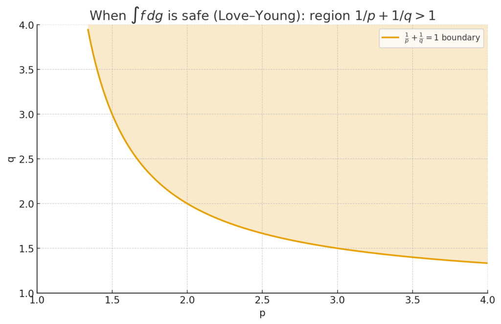
The Love–Young “safe integration” region where $\frac{1}{p}+\frac{1}{q} > 1$ .Example: Brownian needs $p > 2$ ; pair it with something with, say, $q < 2$ so the inequality holds.

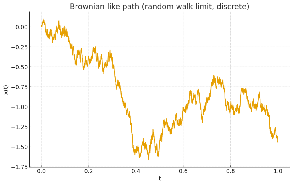
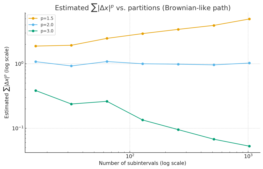
how the estimate $\sum |\Delta x|^p$ changes as we cut the interval into more and more pieces.

Brownian-like path

p=3 shrinks → for $p>2$ , the roughness is “tamed,” and p-variation is finite.

p=1.5 grows with refinement → too rough: p-variation “blows up” for $p\le 2$ .

p=2 hovers around a constant (the borderline).

October 7, 2025

Sonification of the human genome

We applied a Hidden Markov Model to the 1 million exomes from the Regeneron Genetics Center and the 250 thousand exomes from the United States AllofUS project in order to identify regions of the genome that were likely to be constrained and to assign a probability of constraint to each position in the genome.

Dr. Scott Oshiro, a postdoc in the laboratory, with background in music theory and quantum computing decided to sonify constraint in the genome across these two cohorts.

Sonification is the mapping or conversion of data to audio and/or musical elements. For example, a collection of sensor data can be mapped to represent the frequency or pitch of a musical pattern, or its rhythm. This audio file is the sonification of 64 sequences of the human genome. For each genetic sequence there is a value between 0 and 1 representing the probability of a mutation for that particular sequence. These values are mapped to specific pitches for a particular musical scale.

A lot of information is compressed in wave data and I’m excited about the next iteration of our project.

February 22, 2025

Author: admin

Brownian motion and martingales and their relations

Brownian motion

Martingales

Concrete functional analysis

Sonification of the human genome