Manuel A. Rivas and the Rivas Lab

A variant protects against several coronary diagnoses. Another has a large effect on macular degeneration. A third changes metabolic disease risk in opposite directions. Which of these effects should we call localized?

That question matters when we move from a genetic association to a biological hypothesis. A concentrated disease profile may point to a shared process across related diagnoses. A distributed profile can expose connections between systems, including tradeoffs that deserve attention in target discovery. Both are useful. We need to say precisely what the data support.

In SPHERE, we represent phenotype association profiles as fields on a sphere and summarize their spatial structure with spherical harmonics. The maps make concentrated and broad patterns visible. We have now added a complementary comparison that works directly with complete effect estimates and standard errors for a fixed disease panel. It asks whether a disease family has an effect beyond a broad background, then asks how tightly we can bound effects outside that family.[1]

The examples are the best way to see why these questions differ.

From a striking map to a complete phenotype profile

Our archived additive catalogue contains 15,047 variants, 2,349 phenotypes and 35,119 reported variant–phenotype pairs. That is only 0.0994% of the possible matrix. A missing cell in this selected catalogue is an unreported estimate, not evidence of a zero effect.

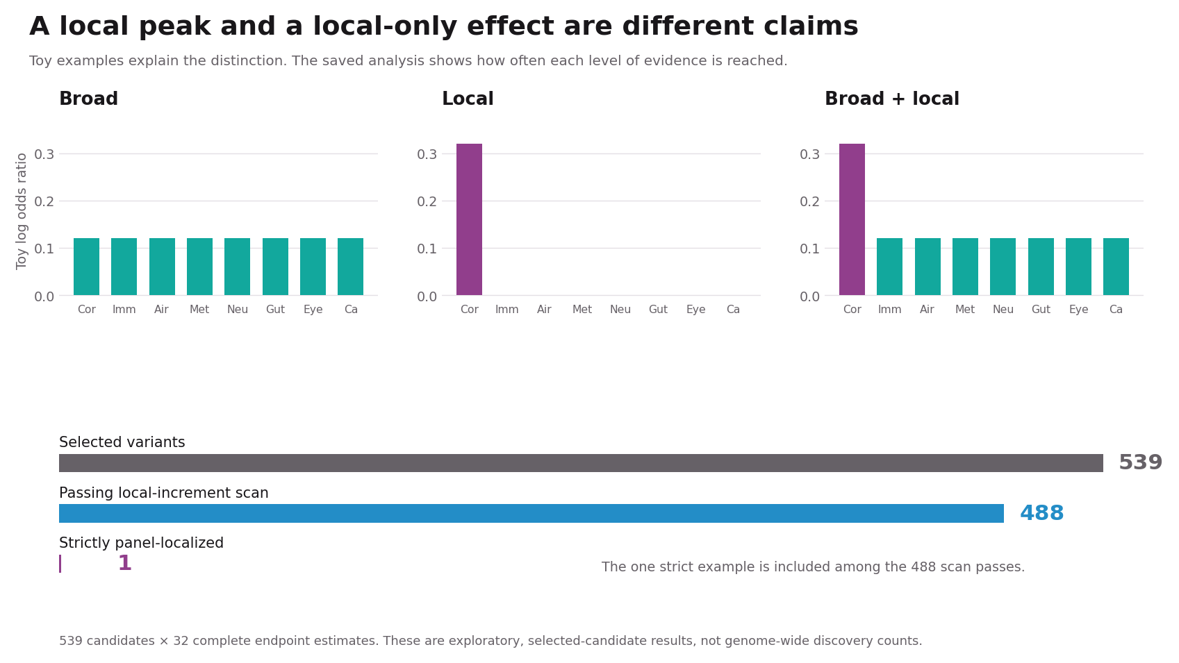
For the new comparison, we retrieved unthresholded effect estimates and standard errors for 539 selected variants across 32 binary endpoints. Four endpoints belong to each of eight families: coronary disease, inflammatory disease, airways, metabolic disease, neurological disease, digestive and biliary disease, eye disease, and cancer. Every candidate has all 32 estimates, giving 17,248 pairs. More than 12,000 of those estimates have original P values of at least 0.05.

Completing the panel makes the outside-effects question possible. It does not erase candidate selection, cover all phenotypes, or turn this into a genome-wide discovery experiment.

Two questions, two levels of evidence

The local-increment test compares a broad phenotype pattern with a model that also allows a family-specific addition. For intuition, start with a constant background and add an effect to the four coronary endpoints. The actual model can accommodate signed broad patterns, so broad effects need not have the same direction in every family. An omnibus family test also permits the four inside endpoints to differ in direction.

A passing local scan establishes a departure from the chosen broad model. It does not establish that outside effects are small. For a stricter label, we additionally choose a margin of log(1.10), approximately 0.0953 in log-odds units. At least one inside effect must be demonstrably larger than that margin, while all 28 outside effects must be bounded below it in magnitude. The bounds use simultaneous intervals across the 32 endpoints for a fixed variant.

Thus “panel-localized” means evidence for a meaningful inside effect and sufficiently small measured outside effects, conditional on this panel, margin and uncertainty model. It does not mean biological effects exist nowhere else.

MFGE8: a coronary pattern that is easy to recognize

The MFGE8 insertion rs534125149 is a particularly compelling starting point. Previous work associated the insertion with protection against coronary atherosclerosis and related diagnoses. That clinical coherence gives the map a biological interpretation: several endpoints may reflect a shared vascular process.[2] The insertion is not established here as a loss-of-function allele, and a protective association alone does not establish the consequences of inhibiting the protein.

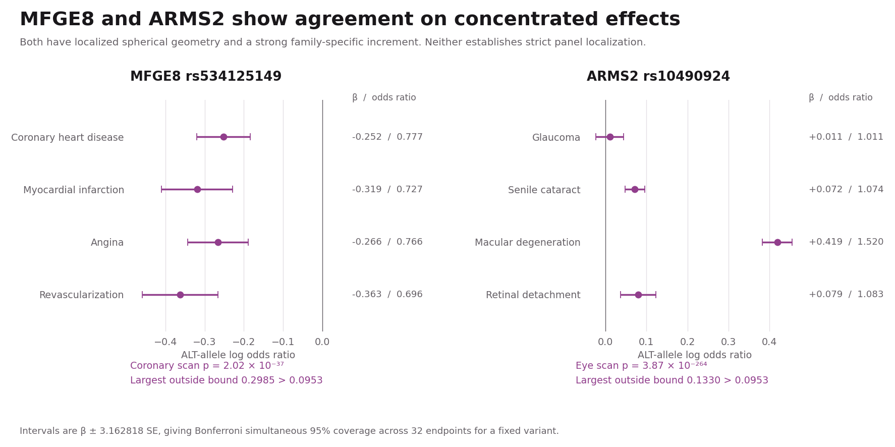
In the saved 32-endpoint profile, the insertion has negative log-odds effects for coronary heart disease, myocardial infarction, angina and coronary revascularization. The corresponding odds ratios are approximately 0.78, 0.73, 0.77 and 0.70. These are related diagnoses moving in a consistent direction, rather than a peak driven by one isolated endpoint.

SPHERE gives this variant a concentrated fitted field: effective area 0.130 and 10-degree cap energy enrichment 12.63-fold. The complete-panel comparison also identifies a coronary-family increment, with within-variant scan-adjusted P approximately 2.02 × 10⁻³⁷.

The stricter outside-effects claim fails. The largest outside upper bound is 0.2985, above the 0.0953 margin. Part of the problem is uncertainty: the bronchiectasis estimate is −0.0492 with standard error 0.0788. There are also nonzero estimates outside the coronary family, including obesity at +0.1063. The correct conclusion is strong agreement on coronary concentration and a local increment. We cannot establish small effects across every measured outside endpoint.

ARMS2: an eye peak that still does not prove exclusivity

The ARMS2-annotated rs10490924 provides a second agreement example. It is the A69S variant at the well-known 10q26 age-related macular degeneration susceptibility locus.[3] This background makes the eye-family peak interpretable, while leaving regional fine-mapping and effector-gene questions open.

In this panel, the macular-degeneration endpoint has log-odds effect +0.4188, an odds ratio of about 1.52. Cataract and retinal-detachment estimates are smaller, at +0.0715 and +0.0794. The four-endpoint omnibus therefore allows a much stronger macular signal alongside weaker or near-zero effects within the same family.

The fitted spherical field is concentrated, with effective area 0.285 and cap enrichment 7.48-fold. The eye-family scan is exceptionally strong, approximately 3.87 × 10⁻²⁶⁴. Yet the outside upper bound is 0.1330, again above the strict margin. A highly significant inside association cannot compensate for insufficiently tight bounds elsewhere. This is why we retain the label “local increment.”

GCKR: one locus, several metabolic directions

GCKR rs1260326 makes the broad-plus-local category biologically intuitive. Earlier studies of the Pro446Leu locus documented opposing glucose and triglyceride associations.[4] Those quantitative traits are external biological context, not endpoints used to produce our 32-disease classification.

The saved results are oriented to the ALT C allele. Type 2 diabetes has a positive log-odds estimate of +0.0549, while lipoprotein disorders and hypercholesterolemia have estimates of −0.0560 and −0.0557. Obesity is close to zero. Averaging these four metabolic endpoints into one signed number would conceal much of the structure.

The covariance-aware metabolic family mean is only 0.004, with standard error 0.005. The common signed-shift test has an unadjusted P value of about 0.045, because positive and negative effects largely cancel. The omnibus metabolic increment is strong, with scan-adjusted P approximately 7.51 × 10⁻³⁸. The distributed broad screen also passes, at P = 0.00870. Outside the metabolic family, the profile includes gallstone disease at +0.0673 and inflammatory bowel disease at −0.0663. SPHERE nevertheless classifies the fitted field as localized, with effective area 0.338.

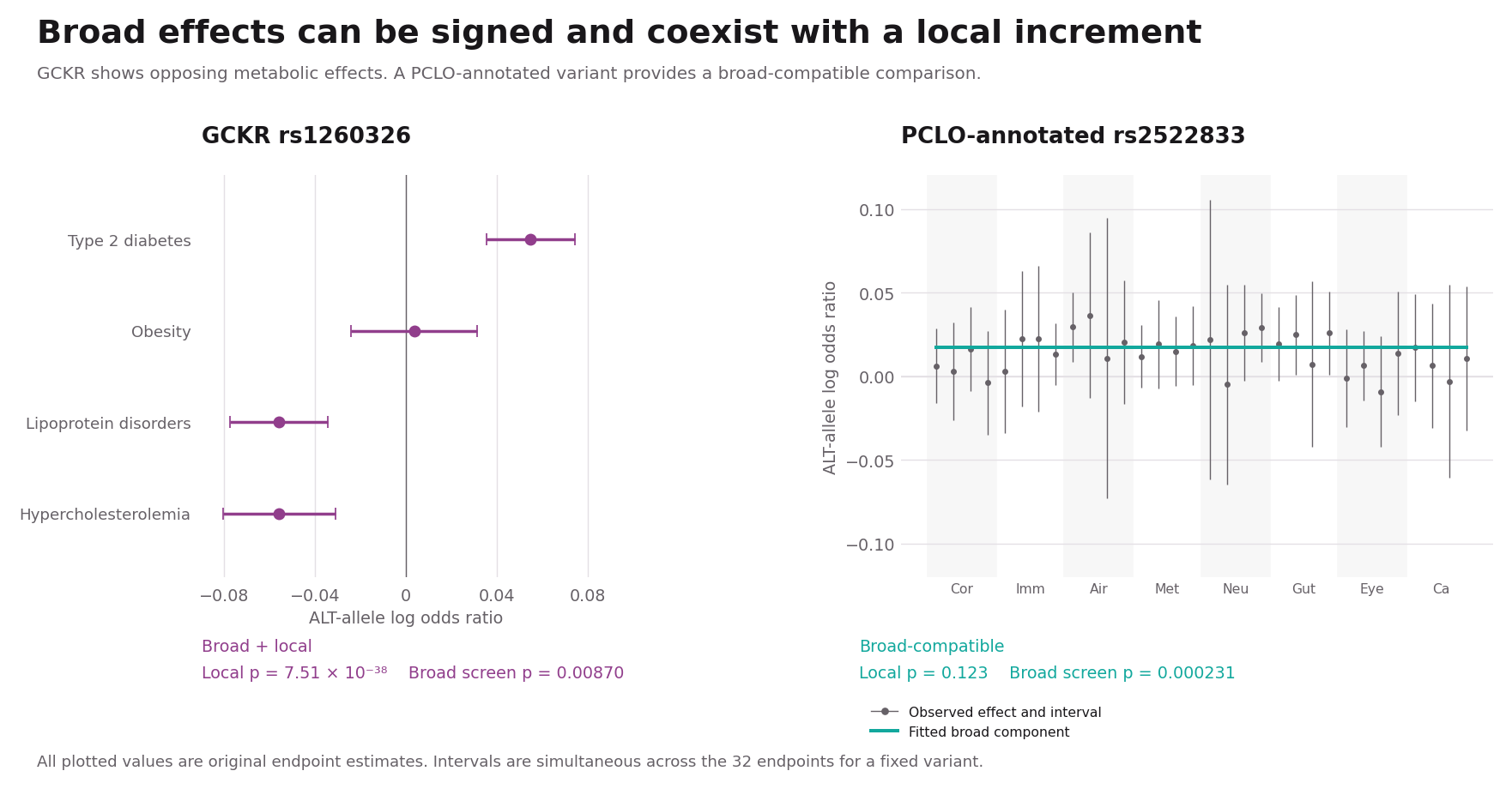
This is an informative difference between the summaries. A concentration measure describes how fitted signal is distributed over the atlas. A distributed-evidence screen asks whether effects are supported across multiple outside families. A variant can satisfy both. For biological interpretation, we should keep the metabolic peak and the wider pattern in view.

The PCLO-annotated rs2522833 supplies a useful broad-compatible comparison: its distributed screen passes at P = 0.000231, while its local scan does not, at P = 0.123. This describes supported distribution across measured families without a detected family increment under the chosen model. It is not a universal pleiotropy verdict.

F5: a disagreement caused by the questions we did not measure

Factor V Leiden, rs6025, is a useful stress test for any comparison of methods. Its association with activated protein C resistance provides a direct coagulation mechanism.[5]

The spherical catalogue profile is localized and coagulation-centered. The 32-endpoint comparison is unresolved, with scan-adjusted P = 0.0553. It would be tempting to treat this as a failed replication of localization. But this fixed panel contains no coagulation family. It cannot directly interrogate the phenotypes that make F5 compelling.

F5 therefore teaches a design lesson: a complete panel can still be incomplete for a particular biological question. The 32 estimates are all present, but the relevant outcomes are absent. A fairer follow-up would prespecify a broader panel including thrombotic and coagulation endpoints and then repeat the analysis.

IL7R: broad geometry can coexist with a local contrast

IL7R rs6897932 illustrates the reverse comparison. Its fitted field has effective area 0.901 and meets the spherical broad criteria. The variant also has established functional context: prior work linked it to IL7R splicing and multiple sclerosis.[6]

In the complete panel, however, the winning contrast is a positive cancer-family increment relative to the fitted broad background, with scan-adjusted P approximately 4.06 × 10⁻¹¹. The saved broad model predicts a cancer-family baseline of −0.0347; the common signed addition is +0.0623. The raw cancer estimates are much smaller, between +0.0147 and +0.0374. Several immune and airway estimates are negative, whereas the cancer estimates are positive. Changing the broad basis could change which family wins this comparison. None of the cancer endpoints establishes an inside magnitude beyond the strict 10% margin under the simultaneous intervals. The outside bound also fails.

The result is a local increment, not strict cancer localization. It does not establish a new cancer-specific mechanism for IL7R or make the prior immune biology irrelevant. It shows how the same profile can have broad spatial structure and a detectable relative departure in one measured family.

POU5F1B: the strongest specificity example in this panel

The POU5F1B-annotated rs6998061 at 8q24 is the only candidate that meets the strict panel-localization rule in the saved run. The locus has prior prostate and colorectal cancer association evidence, so this is not a claim to have discovered a new cancer locus.[7] The annotation also does not establish POU5F1B as the causal gene.

The ALT A allele has log-odds estimates of −0.1532 for prostate cancer and −0.0958 for colorectal cancer, corresponding to odds ratios of approximately 0.86 and 0.91. Breast cancer is +0.0299 and non-small-cell lung cancer is −0.0372. These four cancers should not be collapsed into a claim of uniform protection. The omnibus family test preserves their different effects and yields scan-adjusted P approximately 7.83 × 10⁻³⁷.

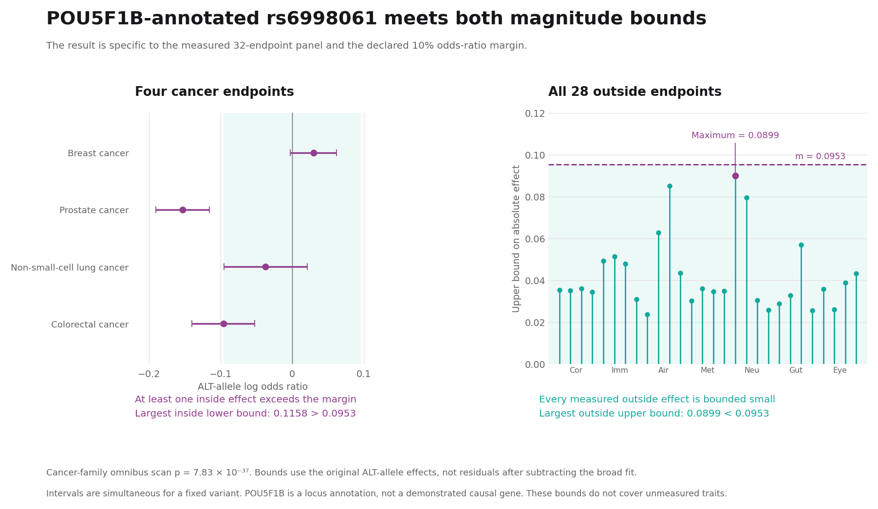
What makes this example special is the outside evidence. The strongest inside lower magnitude bound is 0.1158, beyond the 0.0953 margin. The largest upper magnitude bound across all 28 non-cancer endpoints is only 0.0899, below that margin. The prostate association supplies the decisive inside bound. Every measured outside endpoint clears the corresponding small-effect requirement.

SPHERE assigns this variant to “neither,” which includes support-filter exclusions and intermediate shapes. Only 10 catalogue endpoints are reported, below the geometric classifier’s minimum support of 15. Its fitted shape also does not meet the localization thresholds. This is therefore an informative difference in coverage and estimand, not a clean demonstration that one method has made a false-negative error.

What did the complete comparison find?

Among the 539 preselected candidates, 488 pass the local-increment scan. The exclusive labels are 473 local increments, 14 broad plus local, one panel-localized, four broad-compatible, five dispersed-hit profiles and 42 unresolved. Thus a local departure is common in this selected set, while the stronger outside-bounds requirement is demanding.

An additional covariance-shrinkage sensitivity leaves 505 of 539 labels unchanged. That stability is useful, but it is not full validation. The reference correlation is an estimated proxy that may include genetic signal. Conditional simulations check the local scan with fixed known nuisance quantities, not the entire estimated-nuisance classification pipeline. The within-variant scan correction covers eight families and two test forms. It does not itself correct across the 539 selected candidates.

Using the maps and the presentation together

The presentation follows the same sequence: toy profiles, the measured panel, nested models, uncertainty bounds, then the empirical cases. For each variant, ask three questions. Which diagnoses drive the pattern? What does each method actually summarize? Which additional measurements would strengthen the biological interpretation?

The website provides the maps, comparison tables and exports needed to inspect those answers. We see the greatest value in using spatial structure to organize hypotheses and complete effect profiles to test stronger statements about specificity. A convincing inside signal and informative outside bounds contribute different pieces of evidence. Keeping both visible makes the biology more useful.

Explore the SPHERE method comparison: https://sphere-phenome-atlas.marivascruz.chatgpt.site/method-comparison/

Open the companion presentation (ChatGPT access may be required)

Methods and provenance

All numerical case studies and counts above come from the saved SPHERE comparison summarized in the updated manuscript dated 8 November 2026. The teaching walkthrough uses a fixed broad basis for clarity. The empirical results retain the saved estimated basis and covariance proxy and have not been rerun under a replacement basis. The chromosome-exclusion choice used for nuisance estimation in that saved fit is not a definition of phenotype localization, independent replication, or a calibration guarantee. Simultaneous endpoint bounds apply to a fixed variant under working normal approximations. Prior candidate ascertainment and uncertainty in estimated nuisance quantities remain limitations.

References

[1] SPHERE preprint and the current comparison implementation. Original preprint: https://doi.org/10.1101/2025.10.27.684843 . The November 2026 comparison results discussed here are saved exploratory work associated with the current Site and updated manuscript, not a claim that the original preprint contained this complete analysis.

[2] Ruotsalainen et al. Inframe insertion and splice site variants in MFGE8 associate with protection against coronary atherosclerosis. Communications Biology (2022). https://doi.org/10.1038/s42003-022-03552-0

[3] Kanda et al. A variant of mitochondrial protein LOC387715/ARMS2, not HTRA1, is strongly associated with age-related macular degeneration. PNAS (2007). https://doi.org/10.1073/pnas.0703933104

[4] Orho-Melander et al. Common Missense Variant in the Glucokinase Regulatory Protein Gene Is Associated With Increased Plasma Triglyceride and C-Reactive Protein but Lower Fasting Glucose Concentrations. Diabetes (2008). https://doi.org/10.2337/db08-0516

[5] Bertina et al. Mutation in blood coagulation factor V associated with resistance to activated protein C. Nature (1994). https://doi.org/10.1038/369064a0

[6] Gregory et al. Interleukin 7 receptor alpha chain (IL7R) shows allelic and functional association with multiple sclerosis. Nature Genetics (2007). https://doi.org/10.1038/ng2103

[7] Cavazos et al. Assessment of genetic susceptibility to multiple primary cancers through whole-exome sequencing in two large multi-ancestry studies. BMC Medicine (2022). https://doi.org/10.1186/s12916-022-02535-6